Week 3: Excel Continued & Data Validation & Graphs
Data Validation
Data Validation is a very important aspect in any data entry program. There are a few that we will learn and implement in Excel. They are:
- Range Checking
- Creating Alerts
- Data Type checking
- Restricting Data Entry
- Range Checking:
Excel also allows you to do this.
Exercise 6: [To be submitted]
1. Open the following file:
| datavalidation.xlsx |
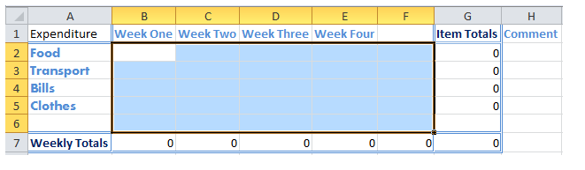
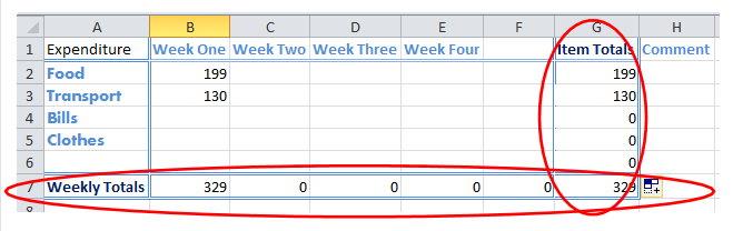
You will see an expenditure list.
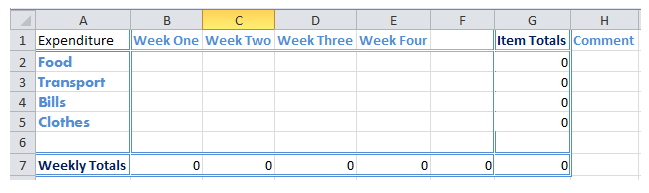
What we want is to have excel not allow the user to enter any value that is greater than our weekly budget $100.
2. Select cell B2
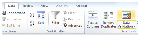
3. Then click on the Data tab, and the Data Validation button.
2. Select cell B2
3. Then click on the Data tab, and the Data Validation button.
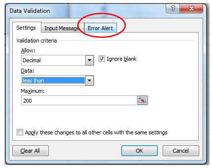
You should get a pop window like below:
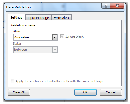
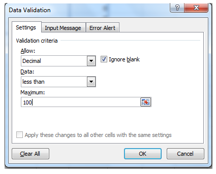
4. Enter the details below:
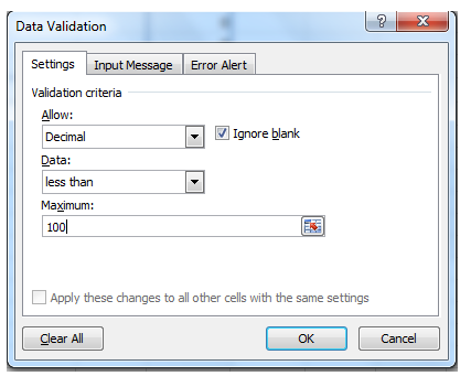
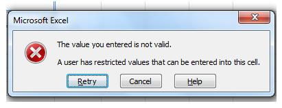
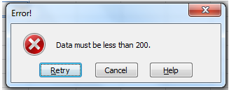
5. Then click ok. This will not allow the user to enter in cell B2 any value greater than 100.6. Type in B2 the value 200 and see what happens.
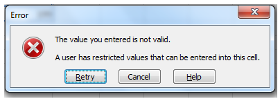
You should get an error like the following:
You should get an error like the following:
6. Select cells between B2 and F6 and make sure they all have a data validation of less than 200.
7. Your turn: Include another type of data validation on your spreadsheet. This could be anything that you think you could add that is relevant.
Creating Alerts
The error message that you had display in the above example - doesn’t tell the user much. If you were to give this file to an employee, they might sit there, looking at the error message wondering what they had done wrong…
To make our excel file more user friendly - we are going to display a proper error message.
To make our excel file more user friendly - we are going to display a proper error message.
- Select cells B2 to F6 again. Then click on the Data tab and the Data Validation option.
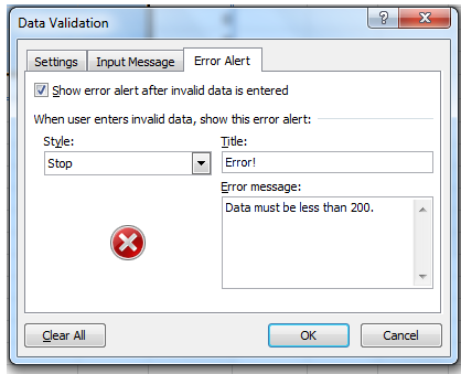
- Click on the Error Alert tab.
3. Then enter in a Title and an Error Message like below:
4. Click ok, then try entering a value in any cell between B2 and F6 that is greater than 200.
You will now see a more informative error message.
You will now see a more informative error message.
Now what if we wanted to stop the user from making this error in the first place?
We can provide the user a bit more information before they enter the value by creating an input message.
5. Select cells B2 to F6. Click on the Data Validation option.
6. Then select the Input Message tab.
We can provide the user a bit more information before they enter the value by creating an input message.
5. Select cells B2 to F6. Click on the Data Validation option.
6. Then select the Input Message tab.
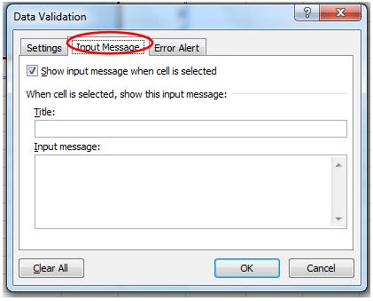
7. Here you can type in a Title and an Input Message like below:
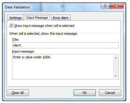
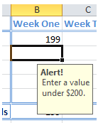
8. Now if you click in any of these cells you will see an input message.
9. In cell B3, enter in the letter 'r' and press enter. You should see an error message.
This is because in our settings we selected 'Decimal' - restricting the data type as a decimal only.
What if we didn’t want our user to change or modify the formula or data in the Weekly Totals and Item Totals for security reasons?
At the moment the file allows anyone to change the formula… if we didn’t have validation rules on our Week 1-4 amounts and I wanted to cheat my budget, in the item total I can change it to subtract $100… thus giving the impression I didn’t spend all that money on Playstation games…
This could create issues in companies and even if the user accidentally deletes something, our data would be incorrect.
To avoid this, we are going to ensure that unless the user has authorisation with a password, they are unable to edit cells G1:G7 and cells A7:G7
Firstly let me use a little analogy to make you understand the next few steps.
Imagine an open door, that is locked. If you close the door - you wont be able to open it again.
This is the settings excel currently has on all cells, the door is currently open, allowing us to make changes to any cells. However, if we lock the door, this means all are cells will be locked, not just the cells we need locked.
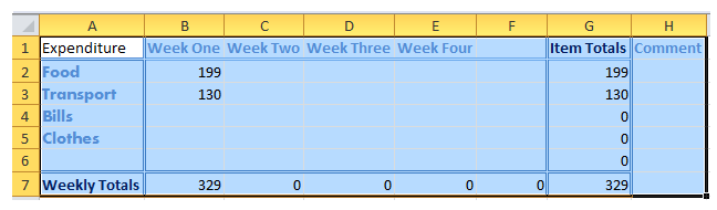
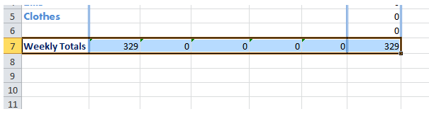
10. Highlight all our cells that we are using in our excel file:
This could create issues in companies and even if the user accidentally deletes something, our data would be incorrect.
To avoid this, we are going to ensure that unless the user has authorisation with a password, they are unable to edit cells G1:G7 and cells A7:G7
Firstly let me use a little analogy to make you understand the next few steps.
Imagine an open door, that is locked. If you close the door - you wont be able to open it again.
This is the settings excel currently has on all cells, the door is currently open, allowing us to make changes to any cells. However, if we lock the door, this means all are cells will be locked, not just the cells we need locked.
10. Highlight all our cells that we are using in our excel file:
11. Then Click on the little arrow in the Number section.
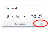
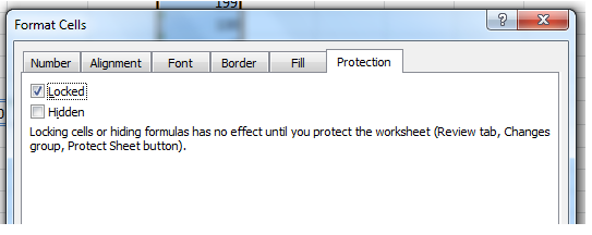
12. Then select the Protection Tab.
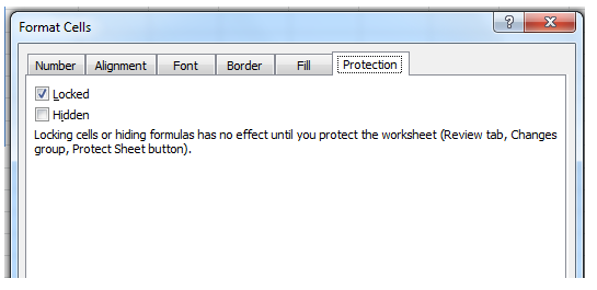
As you can see the cells are all locked… but the door is still open.
We need to unlock all our cells first, then only lock the cells we don’t want the user to modify.
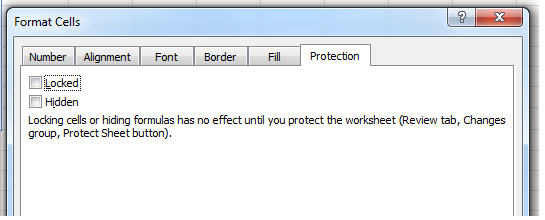
13. Uncheck Locked and click ok.
We need to unlock all our cells first, then only lock the cells we don’t want the user to modify.
13. Uncheck Locked and click ok.
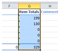
14. Now select cells G1:G7
15. Right click and Select Format Cells
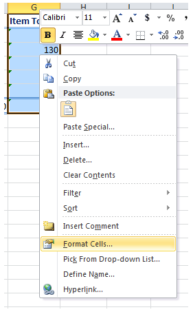
16. Select the Protection Tab again and then check Locked.
Then click ok.
17. Do the same for cells A7:G7
17. Do the same for cells A7:G7
At this point you can still change the values …. Why? Remember our door is still open… even though it is locked. We need to close the door!
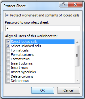
18. Click on the Review Tab and then select Protect Sheet
18. Click on the Review Tab and then select Protect Sheet
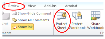
Here is where we close the door and make sure that unless a password is entered, the user can no longer make changes to the data or the formulas in the selected cells.
19. Enter '1' for the password. Make sure that locked and unlocked cells are selected then click ok.
19. Enter '1' for the password. Make sure that locked and unlocked cells are selected then click ok.
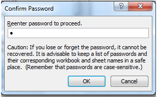
20. Excel will prompt your to re-enter your password. Type '1' again.
Now if you try to enter data in those selected cells or change the formula - you will get an error message.
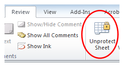
21. As the creator - to be able to change these cells or formulas - all you need to do is unprotect the sheet and enter your password.
21. As the creator - to be able to change these cells or formulas - all you need to do is unprotect the sheet and enter your password.
22. Save your files and Ex6YourName.xlsx and submit.
Exercise 7: [To be submitted]
1. Open the following file:
| ex7.1.xlsx |
2. There are rules at the side of the file listed.
Change the file to follow these rules when entering in data. Ensure you have input & error messages for the user.
3. Protect you worksheets, so that the data in the Price list can not be changed, and the Total column cannot be changed. As a standard for exercises and your outcomes - use '1' as your password.
4. Save your work as Ex7YourName.xlsx and submit.
Creating Graphs
Excel, as you may have noticed has many different ways to present your data graphically.
Here we will look at where to make a graphical representation of your data, how to modify this graph and some handy tips.
1. Open the following file:
Here we will look at where to make a graphical representation of your data, how to modify this graph and some handy tips.
1. Open the following file:
| world_sales.xlsx |
2. Here you will see a simple list of countries and months of world sales. Highlight all the cells including the headings. Don’t forget the headings!!
3. Then click on the Insert Tab on the ribbon
3. Then click on the Insert Tab on the ribbon
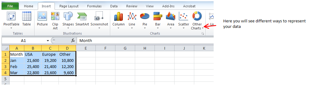
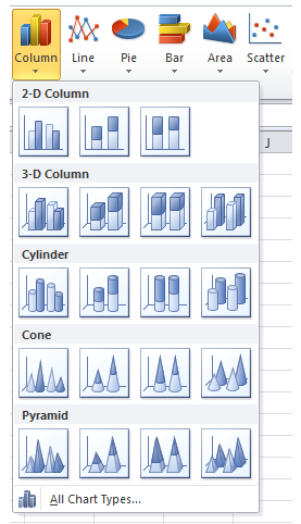
4. You can explore these different graphical representations later, but for now select the Column Chart option.Here you will get a variety of different column charts. Select the 2D clustered column chart for now.
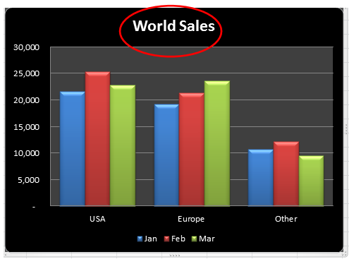
5. You should see the chart below:
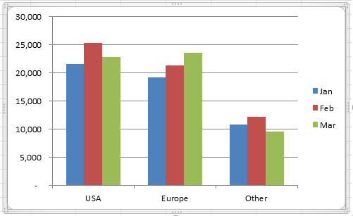
Can you explain what the data shows in this graph?
6. As you can see - excel will automatically open the Design tab for you in the ribbon. There are three Chart Options you will see when you have your graph selected. These are the Design, Layout and Format tabs
6. As you can see - excel will automatically open the Design tab for you in the ribbon. There are three Chart Options you will see when you have your graph selected. These are the Design, Layout and Format tabs
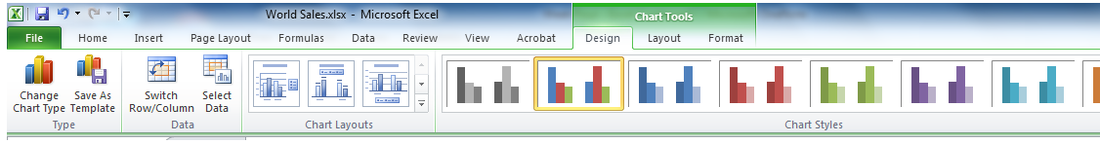
Explore these options and list what they do:
7. Another handy tip to know when it comes to presenting your graph, is the Themes option in the Page Layout tab on the ribbon.
7. Another handy tip to know when it comes to presenting your graph, is the Themes option in the Page Layout tab on the ribbon.
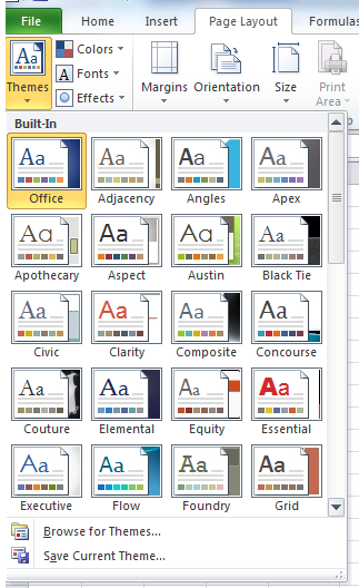
Test out the different themes and see how easy it is to change your graph's appearance.
8. Remember that our graph is dynamic! Meaning that if you change the values in your table data - the graph will update automatically!
9. Click once on the Chart Title to change the Text to World Sales.
8. Remember that our graph is dynamic! Meaning that if you change the values in your table data - the graph will update automatically!
9. Click once on the Chart Title to change the Text to World Sales.
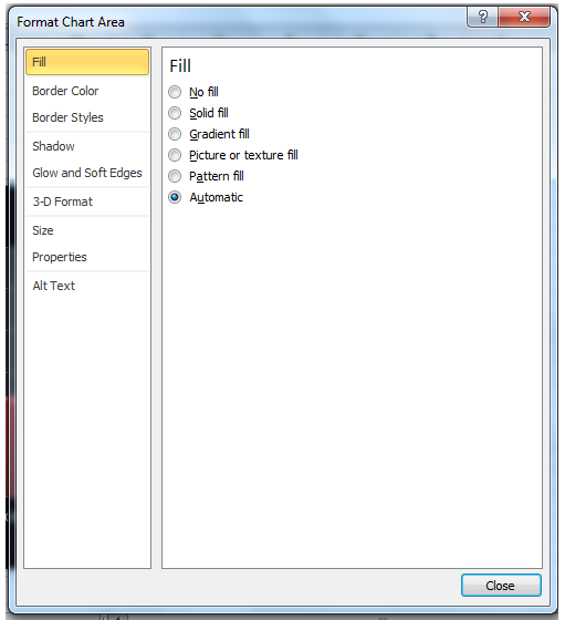
10. Double clicking anywhere on the Graph will open a Properties Window, otherwise known as the Format Chart Area.
Exercise 8: [To be submitted]
What makes a good graphical representation?
How can I improve my presentation? How can I make the data more informative?
How can I improve my presentation? How can I make the data more informative?
Choose from the files below:
| world_sales.xlsx |
| report-login.csv |
1. Using either of the above files, Create a Graphical Representation in either Excel or Piktochart.
Remember to incorporate the skills you have learnt through including functions prior to creating your Graphical Representation.
2. Save as your file and show it to the class.
Remember to incorporate the skills you have learnt through including functions prior to creating your Graphical Representation.
2. Save as your file and show it to the class.
